

The zoo is one of the tourist attractions not just for kids but for all people. These places are public exhibition facilities for wild animals and frequently have advanced breeding facilities where endangered animals may be protected and researched. The most challenging problem with this place is the large numbering of the animals that can’t classify with of them should be included like mammals, reptiles etc. Also, it can’t accommodate easily and manually by the zoo keeper since some of them have large size animals and little extinctions so it gives pressure on and stresses on them.
In this blog, we create this study to apply machine learning techniques and another ensemble modeling to forecast the categorization of the animals based on the factors in order to identify different species and animal categories.
ABOUT DATASETS:
At a subtle way, understanding the link between animal traits and class type in the zoo. Mammals, birds, reptiles, Fish, amphibians, bugs, and invertebrates are all included, which is rather significant. There are essentially 16 variables with various qualities to broadly define the animals, demonstrating how to comprehend the link between the characteristics and class type of animals in the zoo in a sophisticated way. This dataset contains 101 species from a zoo, demonstrating how mammals, birds, reptiles, fish, amphibians, bugs, and invertebrates are all represented in some fashion. I required a data source for my project that could supply distinct Traits in the zoo in a subtle way.
Note: For this post, you can download it from on Kaggle Repository. You can do it through Google Collab or Jupyter Notebook.
PROCEDURES:
PART 1: EXPLORATORY DATA ANALYSIS (EDA)
Data scientists use it to examine and explore data sets and highlight their key properties, frequently using data visualization techniques.
Step 1: Read the data and install the packages or libraries.
#Import Packages
import pandas as pd
import numpy as np
from sklearn.impute import SimpleImputer
import seaborn as sns
import missingno as msno
%matplotlib inline
import matplotlib.pyplot as plt
from sklearn.model_selection import train_test_split, GridSearchCV
from sklearn.metrics import mean_absolute_error
import warnings
warnings.filterwarnings('ignore')

#Read the Data
data = pd.read_csv('Epoch_Final.csv')
Step 2: Get an overview of the dataset:
#Insert the Info of the datasets
data.info()
Step 3: Get an overview of the dataset:
#Insert head of the datasets
data.head()

#Insert tail of the datasets
data.tail()
Step 4: Find the summary statistics of the dataset
#Insert description of the dataset
data.describe()

#Insert complete summary of the dataset
data.describe().T
Step 5: Find the total count and total percentage of missing values in each column of the DataFrame and display them for columns having at least one null value, in descending order of missing percentages.
#Visualising and Analysing Missing Values
mask = data.isnull()
total = mask.sum()
percent = 100*mask.mean()
missing_data = pd.concat([total, percent], axis=1,join='outer',
keys=['count_missing', 'perc_missing'])
missing_data.sort_values(by='perc_missing', ascending=False, inplace=True)
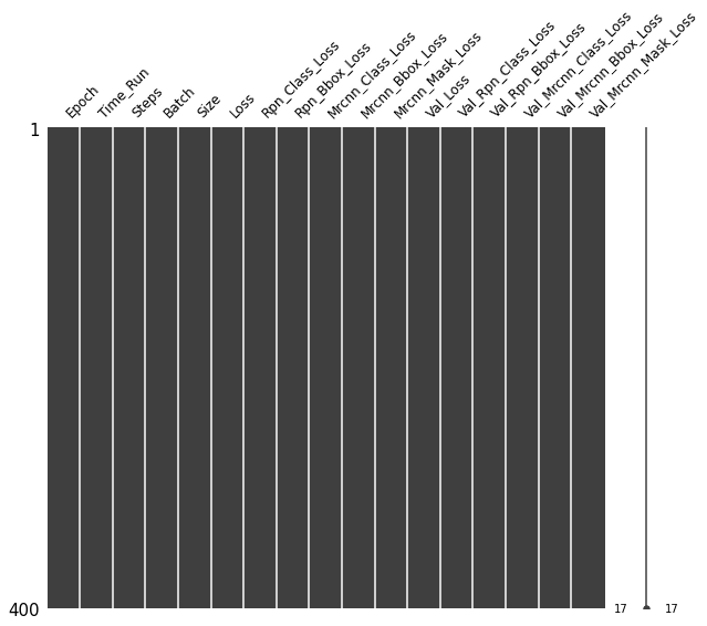
missing_dataStep 6: Plot the nullity matrix and nullity correlation heatmap.
#Plotting Nullity Matrix
msno.matrix(data, figsize=(10,8), fontsize=12)
Output
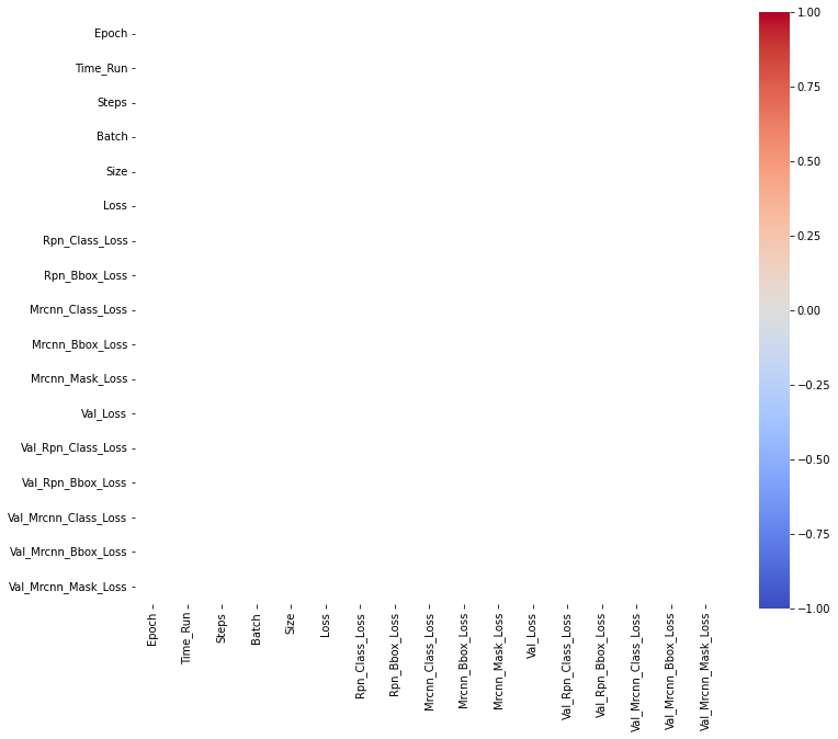
#Plotting Nullity Correlation
plt.figure(figsize=(12,10))
sns.heatmap(data.isnull().corr(),square=True, annot = True, cmap = 'coolwarm', vmin=-1, vmax=1)
plt.show
Output
Step 7: Delete the columns having more than 80% of values missing.
# Since there is no missing columns, there have no reason to use other techniques for the deletion of of the values
# But to check if the columns having more than 80%values missing, Use the Snull Correlation to getter smooth performance.
data.isnull().corr()
Step 8: Impute null values based from the Summary Statistics. Any statistical values can be used for imputation
#Same with the deletion methods columns, this is an optional to use since there is not missing values in this data
#Finding all the numerical variables to replace 0 with randomness value such as mean and std
numeric_variables = data.select_dtypes(include=[np.number])
numeric_variables.columns

#No missing values detected but 0 might be present therefore,
numeric_variables =['Epoch', 'Batch', 'Size', 'Loss', 'Rpn_Class_Loss', 'Rpn_Bbox_Loss',
       'Mrcnn_Class_Loss', 'Mrcnn_Bbox_Loss', 'Mrcnn_Mask_Loss', 'Val_Loss',
       'Val_Rpn_Class_Loss', 'Val_Rpn_Bbox_Loss', 'Val_Mrcnn_Class_Loss',
       'Val_Mrcnn_Bbox_Loss', 'Val_Mrcnn_Mask_Loss']  #declaring the columns that undergo imputation for 0

#Creating def function for imputation of values in terms of 0
def impute_valuemean(f):
  for i in range(0,len(f),2): #impute corresponding mean value in index variables (columns) 0,2,4,6..
    mean = data[f[i]].mean(skipna=True)
    imp = SimpleImputer(missing_values=0, strategy='constant', fill_value=mean)
    data[f[i]] = imp.fit_transform(data[[f[i]]])

#Function for imputation values of corresponding std
def impute_valuestd(x):
  for i in range(1,len(x),2): #impute corresponding std value in index variables(columns) 1,3,5,7..
    std = np.std(data[x[i]])
    imp = SimpleImputer(missing_values=0, strategy='constant', fill_value=std)
    data[x[i]] = imp.fit_transform(data[[x[i]]])

#Imputing missing value using mean value and std value in terms of 0
impute_valuemean(numeric_variables)  #calling function for imputation of missing value using mean in index 0,2,4,6...
impute_valuestd(numeric_variables)   #calling function for imputation of missing value using std in index 1,3,5,7...
data[numeric_variables].info()
Step 9: Visualling and Illustrating the EDA Data
#Sketching Sorting Values
data.skew().sort_values()
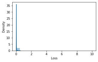
#Visualizing the skewness of the continuous value
plt.figure(figsize=(5,3))
sns.distplot(data.Loss.dropna(), bins=np.linspace(0,10,21))
plt.show()
Output
#Plotting Correlation
plt.figure(figsize=(12,10))
sns.heatmap(data[numeric_variables].corr(),square=True, annot = True, cmap = 'coolwarm', vmin=-1, vmax=1)
plt.show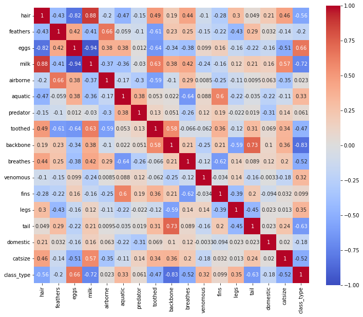
Step 10: OneHotEncoder and Dummy Variable
#Convert all features to numerical values using OneHotEncoder
data.class_type.value_counts()

#Replace the numbers in the class type
data["class_type"].replace([0.0,1.0,4.0],[0,0,0],inplace=True)
data["class_type"].replace([7.0,6.0,5.0],[1,1,1],inplace=True)

#Get dummies of animal names columns
data = pd.get_dummies(data, columns = ['animal_name'])

#Read the data info again with the dummy columns details
data.info()
Step 11: Export the Cleaned Dataset.
#Export the cleaned data
cleaned_data = data
cleaned_data.to_csv('zoo_cleaned.csv')
PART 2: AI MODELLING
Machine learning algorithms that mimic logical decision-making based on available data are developed, trained, and then put into use. Advanced intelligence approaches including real-time analytics, predictive analytics, and augmented analytics are supported by AI models, which act as a foundation.
Note: IF REGRESSION: Use Applied Regression Analysis (ARA) using ENSEMBLE IF CLASSIFICATION: Use Applied Classification Analysis (ACA) using ENSEMBLE. In this session, we are gonna use the ACA method.
Step 1: Import the required dependencies.
#Import Packages for the ACA
from sklearn.linear_model import LogisticRegression
from sklearn.tree import DecisionTreeClassifier
from sklearn.neighbors import KNeighborsClassifier
from sklearn.ensemble import GradientBoostingClassifier, RandomForestClassifier
from sklearn.metrics import f1_score, precision_score, accuracy_score, recall_score
from sklearn.metrics import confusion_matrix, precision_recall_curve, auc, roc_auc_score, roc_curve
from sklearn.ensemble import StackingClassifier
Step 2: Read the cleaned data.
#Read the cleaned data
cleaned_data = pd.read_csv("zoo_cleaned.csv")
Step 3: Divide the dataset into train and validation DataFrames.
#Split the datasets based on the needs for DataFrames
x = data.drop(["class_type"], axis = True)
y = data["class_type"]

#Using the model selection, train and test the data
from sklearn.model_selection import train_test_split
X_train, X_val, y_train, y_val = train_test_split(x, y, test_size = 0.15, random_state = 11)
Step 4: Construct an Ensemble model (STACKING Ensemble) using 2 base classifiers and 1 stacked model as a classifier.
For KNeighbors Classifier
#Use the Hypertuning parameter for KNN
params_knn = {
"leaf_size": list(range(1,30)),
"n_neighbors": list(range(1,21)),
"p": [1,2]
}
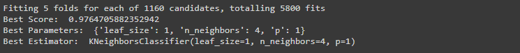
#Perform ensemble model for KNN
grid_search_kn = GridSearchCV(KNeighborsClassifier(), params_knn, verbose=1, cv=5)
grid_search_kn.fit(X_train, y_train);
print ("Best Score: ", grid_search_kn.best_score_)
print ("Best Parameters: ", grid_search_kn.best_params_)
print ("Best Estimator: ", grid_search_kn.best_estimator_)Output:
For Decision Classifier
#Use the Hypertuning parameter for DTC
params_dt = {
'max_leaf_nodes': list(range(2, 100)),
'min_samples_split': [2, 3, 4]
}
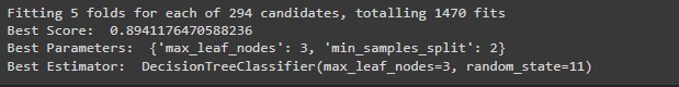
#Perform ensemble model for DTC
grid_search_dt = GridSearchCV(DecisionTreeClassifier(random_state=11), params_dt, verbose=1, n_jobs = -1)
grid_search_dt.fit(X_train, y_train)
print ("Best Score: ", grid_search_dt.best_score_)
print ("Best Parameters: ", grid_search_dt.best_params_)
print ("Best Estimator: ", grid_search_dt.best_estimator_)Output
For Logistics Regression
#Use the Hypertuning parameter for Lr
params_lr = {
"C":np.logspace(-3,3,7),
"penalty":["l1","l2"]
}

#Perform ensemble model for Lr
grid_search_lr = GridSearchCV(LogisticRegression(random_state=11), params_lr, cv=10)
grid_search_lr.fit(X_train, y_train)
print ("Best Score: ", grid_search_lr.best_score_)
print ("Best Parameters: ", grid_search_lr.best_params_)
print ("Best Estimator: ", grid_search_lr.best_estimator_)
Output

Note: You can adjust the code in the 3 classifier according to your datasets;
kn_params = {
'leaf_size': 1,
'n_neighbors': 3,
'p': 1
}

decisiontree_params = {
'max_leaf_nodes': 42,
'min_samples_split': 4
}

lr_params = {
'C': 1.0,
'penalty': 'l2'
}
Step 5: Calculate the accuracy, precision, and recall for predictions on the validation set, and print the confusion matrix (Target F1-Score >= 90%):
#Performance base on accuracy, precision, and recall for predictions on the validation set, and print the confusion matrix for KNN
knn = KNeighborsClassifier(**kn_params)
knn.fit(X_train, y_train)
knnpred_val = knn.predict(X_val)
accuracyscore = accuracy_score(y_val, knnpred_val)
precisionscore = precision_score(y_val, knnpred_val, average='weighted')
recallscore = recall_score(y_val, knnpred_val, average='macro')
f1score = f1_score(y_val, knnpred_val, average = 'micro')
cm_rf = confusion_matrix(y_val, knnpred_val)
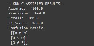
print("--KNN CLASSIFIER RESULTS--")
print("Accuracy: ", accuracyscore*100)
print("Precision: ", precisionscore*100)
print("Recall: ", recallscore*100)
print("F1-Score: ", f1score*100)
print("Confusion Matrix: \n", cm_rf)Output
#Performance base on accuracy, precision, and recall for predictions on the validation set, and print the confusion matrix for DTC
dt = DecisionTreeClassifier(**decisiontree_params, random_state=11)
dt.fit(X_train, y_train)
dtpred_val = dt.predict(X_val)
accuracyscore1 = accuracy_score(y_val, dtpred_val)
precisionscore1 = precision_score(y_val, dtpred_val, average='weighted')
recallscore1 = recall_score(y_val, dtpred_val, average='weighted')
f1score1 = f1_score(y_val, dtpred_val, average = 'micro')
cm_rf1 = confusion_matrix(y_val, dtpred_val)
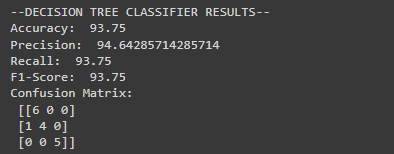
print("--DECISION TREE CLASSIFIER RESULTS--")
print("Accuracy: ", accuracyscore1*100)
print("Precision: ", precisionscore1*100)
print("Recall: ", recallscore1*100)
print("F1-Score: ", f1score1*100)
print("Confusion Matrix: \n", cm_rf1)Output
#Performance base on accuracy, precision, and recall for predictions on the validation set, and print the confusion matrix for Stacked Classifier
estimator_list = [
('knn', knn),
('dt', dt),
]
stacked_model = StackingClassifier(estimators=estimator_list, final_estimator=LogisticRegression(**lr_params))
stacked_model.fit(X_train, y_train)
stacked_preds_val = stacked_model.predict(X_val)
accuracyscore2 = accuracy_score(y_val, stacked_preds_val)
precisionscore2 = precision_score(y_val, stacked_preds_val, average='micro')
recallscore2 = recall_score(y_val, stacked_preds_val, average='micro')
f1score2 = f1_score(y_val, stacked_preds_val, average = 'micro')
cm_rf2 = confusion_matrix(y_val, stacked_preds_val)
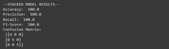
print("--STACKED MODEL RESULTS--")
print("Accuracy: ", accuracyscore2*100)
print("Precision: ", precisionscore2*100)
print("Recall: ", recallscore2*100)
print("F1-Score: ", f1score2*100)
print("Confusion Matrix: \n", cm_rf2)Output
Step 6: Plot the performance accordingly, use the appropriate plotting:
#Replace the few values
y_val.replace([2],[1],inplace=True)

#Predict_Proba using Sci-learn
r_probs = [0 for _ in range(len(y_val))]
knn_probs = knn.predict_proba(X_val)
dt_probs = dt.predict_proba(X_val)
sm_probs = stacked_model.predict_proba(X_val)

#Probs of the classifier
knn_probs = knn_probs[:, 1]
dt_probs = dt_probs[:, 1]
sm_probs = sm_probs[:, 1]

#Plotting score of AUC and ROC
r_auc = roc_auc_score(y_val, r_probs)
knn_auc = roc_auc_score(y_val, knn_probs)
dt_auc = roc_auc_score(y_val, dt_probs)
sm_auc = roc_auc_score(y_val, sm_probs)

#Combined the strucure of AUC-ROC of each classifier
r_fpr, r_tpr, _ = roc_curve(y_val, r_probs)
knn_fpr, knn_tpr, _ = roc_curve(y_val, knn_probs)
dt_fpr, dt_tpr, _ = roc_curve(y_val, dt_probs)
sm_fpr, sm_tpr, _ = roc_curve(y_val, sm_probs)

#Import the matplotlib
import matplotlib.pyplot as plt

#Plotting AUC-ROC for with the Rate
plt.plot(r_fpr, r_tpr, linestyle='--', label='Random Prediction (AUROC = %0.3f)' % r_auc)
plt.plot(knn_fpr, knn_tpr, marker='.', label='KNeighbors (AUROC = %0.3f)' % knn_auc)
plt.plot(dt_fpr, dt_tpr, marker='.', label='Decision Tree (AUROC = %0.3f)' % dt_auc)
plt.plot(sm_fpr, sm_tpr, marker='.', label='Logistic Regression (AUROC = %0.3f)' % sm_auc)
# Title
plt.title('ROC Plot')
# Axis labels
plt.xlabel('False Positive Rate')
plt.ylabel('True Positive Rate')
# Show legend
plt.legend() #
# Show plot
plt.show()
Output
Step 7: Test the final values on the test datasets.
#Results of the Actual and Predicted of the datasets.
results = X_val.copy()
results ['Actual'] = y_val
results ['Predicted'] = stacked_model.predict(X_val)
results = results[['Actual', 'Predicted']]
results[:10]
Step 8: Export the Final Model using PICKLE Library.
## Import pickle library
import pickle
filename = 'Lisboa-Finals'
pickle.dump(stacked_model,open(filename,'wb'))CONCLUSION:
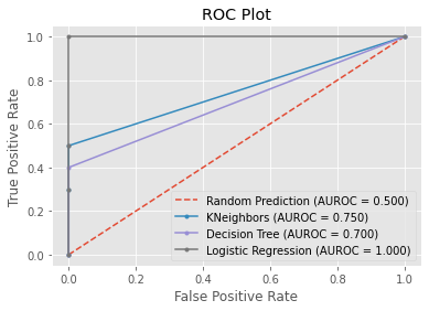
During the process of locating the optimal classification model, valuable insights were obtained. It was possible to classify the different distinct class types of animals with a level of accuracy that was high by making use of sklearn classification models such as KNN and Decision Tree as well as Logistic Regression. Utilizing GridSearchCV allows for the automatic retrieval of the parameter that provides the best results possible. The K-Nearest Neighbors algorithm was given a score of 0.75 on the AUROC, while the Decision Tree algorithm was given a score of 0.70. When it came to accuracy, the Decision Tree model performed significantly better than the KNN model. In conclusion, given that it has an AUROC of 1.0, Logistic Regression should be able to perform well on future samples of the class types of animals for the menagerie and identify them with a high degree of accuracy. Comparison of the machine learning models have existed. The three models, KNN is the longest process of the training the datasets while the Logistics Regression.
This study helps to identify organisms. establish relationship among various group of organisms. By studying a few organisms, the characteristics of the whole group can be understood. These performances were also only achieved by using a dataset that has the potential to be expanded upon in order to broaden its scope and further improve its performance. Moreover, the use of this dataset was the only way that these performances could be achieved.
Reference:
National Geographic Society, “zoo,” National Geographic Headquarters 1145 17th Street NW Washington, DC 20036, 2022. https://education.nationalgeographic.org/resource/zoo (accessed May 31, 2022).
[2] A. M. Godinez and E. J. Fernandez, “What is the zoo experience? How zoos impact a visitor’s behaviors, perceptions, and conservation efforts,” Front. Psychol., vol. 10, no. JULY, p. 1746, 2019, doi: 10.3389/FPSYG.2019.01746/BIBTEX.
[3] E. Dandil and R. Polattimur, “PCA-Based Animal Classification System,” ISMSIT 2018 – 2nd Int. Symp. Multidiscip. Stud. Innov. Technol. Proc., pp. 1–5, 2018, doi: 10.1109/ISMSIT.2018.8567256.
[4] E. Sasmaz and F. B. Tek, “Animal Sound Classification Using A Convolutional Neural Network,” UBMK 2018 – 3rd Int. Conf. Comput. Sci. Eng., pp. 625–629, 2018, doi: 10.1109/UBMK.2018.8566449.
[5] N. K. El Abbadi and E. M. T. A. Alsaadi, “An Automated Vertebrate Animals Classification Using Deep Convolution Neural Networks,” Proc. 2020 Int. Conf. Comput. Sci. Softw. Eng. CSASE 2020, pp. 72–77, 2020, doi: 10.1109/CSASE48920.2020.9142070.
[6] S. Fujimori, T. Ishikawa, and H. Watanabe, “Animal behavior classification using DeepLabCut,” 2020 IEEE 9th Glob. Conf. Consum. Electron. GCCE 2020, pp. 254–257, 2020, doi: 10.1109/GCCE50665.2020.9291715.
[7] L. Prudhivi, M. Narayana, C. Subrahmanyam, and M. Gopi Krishna, “Animal species image classification,” Mater. Today Proc., no. xxxx, 2021, doi: 10.1016/j.matpr.2021.02.771.
[8] A. Ahmed, H. Yousif, R. Kays, and Z. He, “Animal species classification using deep neural networks with noise labels,” Ecol. Inform., vol. 57, no. January, p. 101063, 2020, doi: 10.1016/j.ecoinf.2020.101063.[9] L. Kuncheva, “Animal reidentification using restricted set classification,” Ecol. Inform., vol. 62, no. February, p. 101225, 2021, doi: 10.1016/j.ecoinf.2021.101225.