
In linear regression models, we employ the dummy variable strategy to build a model that can infer a link between features and the result. Dummy variables are categorical variables that we can introduce into a model, using the information provided within the existing dataset. The design and selection of these variables are considered components of feature engineering, and depending upon the choice of variables, the results may vary.
In this blog, we are going to create two categorical variables, one indicating if the year is greater than 1960 and one if the year is greater than 1940. These two years were chosen as limits for creating the dummy variables because of the shape of the 15 year moving average. As discussed there seems to be the start of an increasing trend around 1960 and 1940 was sellected as this is the approximate end of the early plateau.
Note: For this post, the dataset Early Plateau from the statistic platform “Kaggle” was used. You can download it from my GitHub Repository. You can do it through Google Collab or Jupyter Notebook.
Step 1: Loading the libraries and the data
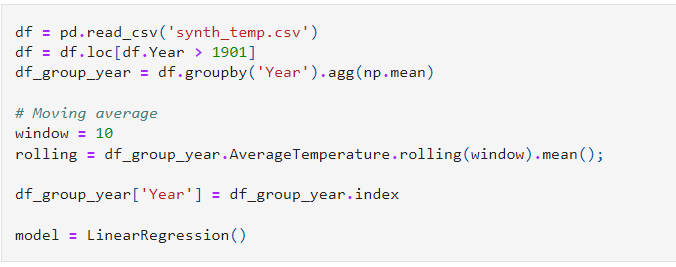
Step 2: Reload the data from the datasets, For convenience, assign the index values of the df_group_year DataFrame to the Year column:
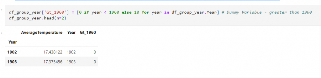
Step 3: Create a dummy variable with a column labeled Gt_1960, where the value is 0 if the year is less than 1960 and 10 if greater:
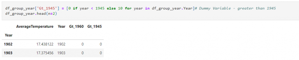
Step 4: Create a dummy variable with a column labeled Gt_1945, where the value is 0 if the year is less than 1945 and 10 if greater:
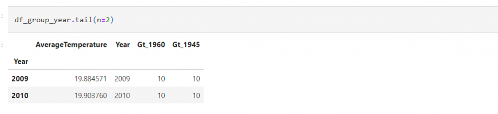
Step 5: Call the tail() method to look at the last two rows of the df_group_year DataFrame to confirm that the post 1960 and 1945 labels have been correctly assigned:
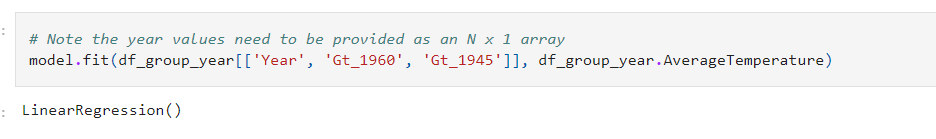
Step 6: Fit the linear model with the additional dummy variables by passing the Year, Gt_1960, and Gt_1945 columns as inputs to the model, with AverageTemperature again as the output:
Step 7: Check the R-squared score for the new model against the training data to see whether we made an improvement:
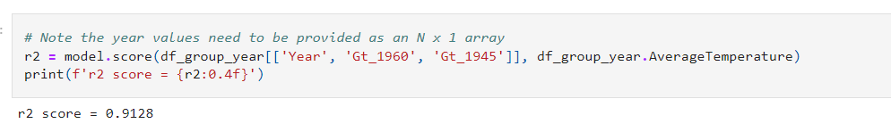
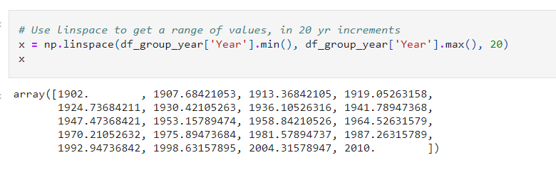
Step 8: We have made an improvement! This is a reasonable step in accuracy given that the first model’s performance was 0.8618. We will plot another trendline, but we will need more values than before to accommodate the additional complexity of the dummy variables. Use linspace to create 20 linearly spaced values between 1902 and 2013:
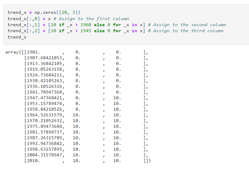
Step 9: Create an array of zeros in the shape 20 x 3 and fill the first column of values with x, the second column with the dummy variable value for greater than 1960, and the third column with the dummy variable value for greater than 1945:
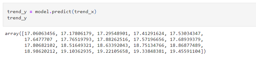
Step 10: Now get the y values for the trendline by making predictions for trend_x:
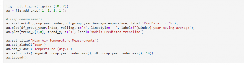
Step 11: Plot the trendline:
Output:
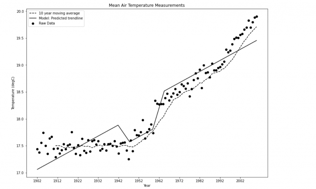
Note: Incorporating dummy variables made quite an improvement to the model, but looking at the trendline, it doesn’t seem like a reasonable path for natural phenomena such as temperature to take and could be suffering from overfitting. We will cover overfitting in more detail in Chapter, Ensemble Modeling; however, let’s use linear regression to fit a model with a smoother prediction curve, such as a parabola.
Conclusion:
Dummy variables have benefits in that they allow us to represent many groups using a single regression equation. As a result, we are relieved of the necessity to create unique equation models for every subgroup. The dummy variables function as “switches” that toggle certain equation parameters on and off.